Speech Dereverberation in the Frequency Domain

For full details, please refer to the paper listed below.

• Y.(Grace) Li, D. Williamson, "A Return to Dereverberation in the Frequency Domain Using a Joint Learning Approach," in Proc. IEEE International Conference on Acoustics, Speech and Signal Processing (ICASSP), pp. 7549-7553, 2020. [PDF]

Abstract

Dereverberation is often performed in the time-frequency domain using mostly deep learning approaches. Time-frequency domain processing, however, may not be necessary when reverberation is modeled by the convolution operation. In this paper, we investigate whether deverberation can be effectively performed in the frequency-domain by estimating the complex frequency response of a room impulse response. More specifically, we develop a joint learning framework that uses frequency-domain estimates of the late reverberant response to assist with estimating the direct and early response. We systematically compare our proposed approach to recent deep learning based approaches that operate in the time-frequency domain. The results show that frequency-domain processing is in fact possible and that it often outperforms time-frequency domain based approaches under different conditions.

Background

Reverberation degrades perceptual speech quality and intelligibility as sound reflections obscure signal structure. This creates a challenge for many applications, including, hearing aids, automatic speech recognition and speaker identification. Dereverberation is often performed in the time-frequency domain using mostly deep learning approaches. Time-frequency domain processing, however, may not be necessary when reverberation is modeled by the convolution operation. As an alternative approach to perform dereverberation in frequency-domain with deep learning-based approach, can avoid assumptions to hold in different environments.

Algorithm Description

1. Problem formulation:
The objective is to remove the late reflections from the corresponding reverberant speech signal by operating in the frequency domain. The prediction target is direct plus early room impulse response (RIR) in frequency domain. The network using is joint-LSTM network to predict both direct plus early RIR and late RIR in frequency domain.

2. Features:
Given a time domain reverberant signal y(t): compute the 1024-point discrete Fourier transform (DFT); concatenate the real and imaginary components of the 1024-point DFT as input.

$Y(m)=\left[\begin{array}{1}{Y_{i}(i) Y_{i}(2) \dots Y_{i}(N)} \\ {Y_{r}(1) Y_{r}(2) \dots Y_{r}(N)}\end{array}\right]$

$Y = \{Y(1) Y(2) \cdots Y(N_S)\}$

3. Training Labels:
Predict transfer functions of the RIRs instead of speech: transform the direct plus early RIR ($h_{de}(t)$) and the late RIR ($h_{l}(t)$) into 1024-point DFTs (N = 1024); concatenate the real and imaginary components of the resulting DFT into one.

$H_{l}(m) = \{H_{l}(1) H_{l}(2) \cdots H_{l}(N)\}$

$H_{de}(m) = \{H_{de}(1) H_{de}(2) \cdots H_{de}(N)\}$

4. Objective Function:
Trained using standard back propagation algorithm with mean-square error cost function

$$\frac{1}{2 N} \sum_{f}\left[\left(\widehat{H}_{l}^{r}(f)-H_{l}^{r}(f)\right)^{2}+\left(\widehat{H}_{l}^{i}(f)-H_{l}^{i}(f)\right)^{2}\right] $$

$$+ \frac{1}{2 N} \sum_{f}\left[\left(\widehat{H}_{d e}^{r}(f)-H_{d e}^{r}(f)\right)^{2}+\left(\widehat{H}_{d e}^{i}(f)-H_{d e}^{i}(f)\right)^{2}\right] $$

Network Structure

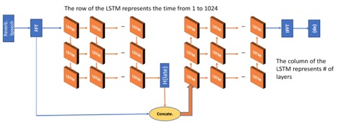
(From left to right)The left part of the network predicts the late RIR in frequency domain: the number of neurons is set to 2048 for each LSTM layer; three fully connected (FCN) layers. The right part predicts the direct plus early RIR in frequency domain: the number of neurons is set to 4096 for first 2 LSTM layers; the number of neurons is set to 2048 for the last LSTM layer; three FCN layers.

Experimental Results

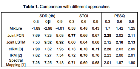
(From left to right) SDR(db) results, STOI (from 0 to 1) results, PESQ (from -0.5 tp 4.5) results. The cIRM, IRM, and Spectral Mapping represent the corresponding systems that are implementing in time-frequency domain, and the Joint FCN and Joint LSTM represent the systems that are implementing in frequency domain. The best result in each category is represented in bold.

×

Speech Enhancement Using Intra-Spectral Recurrent Layers

For full details, please check out the following paper that is referenced below. You can also view the above video by Khandokar Md. Nayem for a general overview of the approach.

• K. M. Nayem and D. Williamson, "Monaural Speech Enhancement Using Intra-Spectral Recurrent Layers In The Magnitude & Phase Responses," in Proc. IEEE International Conference on Acoustics, Speech, and Signal Processing (ICASSP), pp. 6224-6228, 2020. [PDF] [SLIDES]

Abstract

Speech enhancement has greatly benefited from deep learning. Currently, the best performing deep architectures use long short-term memory (LSTM) recurrent neural networks (RNNs) to model short and long temporal dependencies. These approaches, however, underutilize or ignore spectral-level dependencies within the magnitude and phase responses, respectively. In this paper, we propose a deep learning architecture that leverages both temporal and spectral dependencies within the magnitude and phase responses. More specifically, we first train a LSTM network to predict both the spectral-magnitude response and group delay, where this model captures temporal correlations. We then introduce Markovian recurrent connections in the output layers to capture spectral dependencies within the magnitude and phase responses. We compare our approach with traditional enhancement approaches and approaches that consider spectral dependencies within a single time frame. The results show that considering the within-frame spectral dependencies leads to improvements.

Introduction

Monaural speech enhancement is a challenging task that aims to remove unwanted background noise from a single audio channel, to improve perceptual speech intelligently and quality. Deep learning has resulted in improved performance, but additional improvement is needed in noisy environments. An end-to-end model that uses an utterance-based objective function shows promising results in speech enhancement tasks, and it preserves high and low-frequency spectral information. In these approaches, the approximated time-frequency (T-F) output is based on prior network layers and prior (in time) outputs of that T-F unit. The output, however, is not based on the adjacent or nearby frequency points within the magnitude response. It is known, however, that speech has spectral dependencies along the frequency axis, but current architectures often ignore these correlations. In speech recognition [2] and audio restoration after coding [1], dedicated LSTM modules are used to learn spectral dependencies, but this is either done at the subband frequency-level or overall time. Additionally, these approaches do not consider local spectral dependencies over short-time instances. Hence, We propose an intra-spectral (e.g. across-frequency) recurrent layer that captures frequency dependencies within each time frame of a speech signal. Given a noisy speech input, a LSTM network with multiple target loss functions learns the temporal dependencies of speech. We then append the proposed intra-spectral recurrent (ISR) layer to enforce spectral-level dependencies. Our preliminary work showed that incorporating spectral-level dependencies within the magnitude domains leads to noticeable improvements [18].

Magnitude and phase information

In the time domain, noisy speech $m_t$ is a sum of clean speech $s_t$ and noise $n_t$, where $t$ is the time index.

$m_t = s_t + n_t $

Correspondingly, $M_{t,k}$ is the noisy speech in T-F domain, which is the multiplication of magnitude $|M_{t,k}|$ and exponent of phase $e^{i \theta^M_{t,k}}$, here $k$ is the frequency index. We can consider the noisy speech as a union of two sound sources, $𝑆_{𝑡,𝑘}$ which is the clean speech and $𝑁_{𝑡,𝑘}$ which is the noise, in T-F with phase $\theta^S_{t,k}$ and $\theta^N_{t,k}$ respectively.

$\begin{aligned}M_{t,k} &= |M_{t,k}| e^{i \theta^M_{t,k}} \\ &= |𝑆_{𝑡,𝑘}|e^{i \theta^S_{t,k}} \cup |𝑁_{𝑡,𝑘}|e^{i \theta^N_{t,k}}\\ &= S_{t,k} \cup N_{t,k}\end{aligned}$

Our goal is to approximate clean speech $\hat{𝑆}̂_{𝑡,𝑘}$ by learning the function $𝐹_\phi$ on noisy speech, in another word, on magnitude and phase of noisy speech. This can be close approximate to the magnitude and phase responses of clean speech and noise, given that we can separate the sound sources.

$\begin{aligned}\hat{𝑆}̂_{𝑡,𝑘} = 𝐹_\phi(M_{t,k}) =& 𝐹_\phi(|M_{t,k}|, \theta^M_{t,k})\\ \approx& 𝐹_\phi(|𝑆_{𝑡,𝑘}|, |𝑁_{𝑡,𝑘}|, \theta^S_{t,k}, \theta^N_{t,k}) \end{aligned}$

Group delay of signal can be computed as angular exponent of phase difference between $(k+1)$ and $k$-th frequency. Here, we denote Group delay (GD) of signal $𝑆_{𝑡,𝑘}$ as $GD^S_{t,k}$.

$GD^S_{t,k}= \angle e^{i(\theta^S_{t,k+1}-\theta^S_{t,k})} $

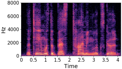
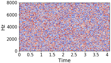
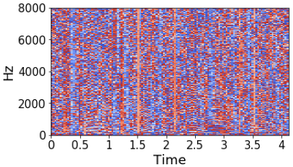
Unlike magnitude response, the phase of a speech does not show a clear structure. As we can see in the following pictures, the left one is a magnitude spectrogram of a signal and middle one is the phase of the speech. Even though, this is a clean speech signal, the phase plot does not show any clear structure. On the other hand, the right most picture which is group delay of the signal shows a learn-able pattern in log-magnitude formulation.

For learning magnitude, the optimal estimated magnitude loss function $\mathcal{L}_{mag}$ is the sum of mean squared error of magnitude between (clean and estimated speech), and between (noise and estimated noise). For learning group delay, optimal estimated group delay loss function $\mathcal{L}_{gd}$ is the sum of cosine distance of group delay between (clean and estimated speech), and between (noise and estimated noise). Therefore, the combined loss function, $\mathcal{L}_{mag+gd}$ is the weighted average of $\mathcal{L}_{mag}$ and $\mathcal{L}_{gd}$.

$\begin{aligned}\mathcal{L}_{mag} =& \sum_{t,k} (|\hat{S}_t,k|-|{S}_t,k|)^2 + (|\hat{N}_t,k|-|{N}_t,k|)^2 \\ \mathcal{L}_{gd} =& \sum_{\chi\in\{S,N\}} \sum_{t,k} |\chi_{t,k+1}| \frac{\big( 1-cos(\hat{GD}^\chi_{t,k}-GD^\chi_{t,k})\big)}{2}\\ \mathcal{L}_{mag+gd} =& \lambda \mathcal{L}_{mag} + (1-\lambda)\mathcal{L}_{gd} \end{aligned}$

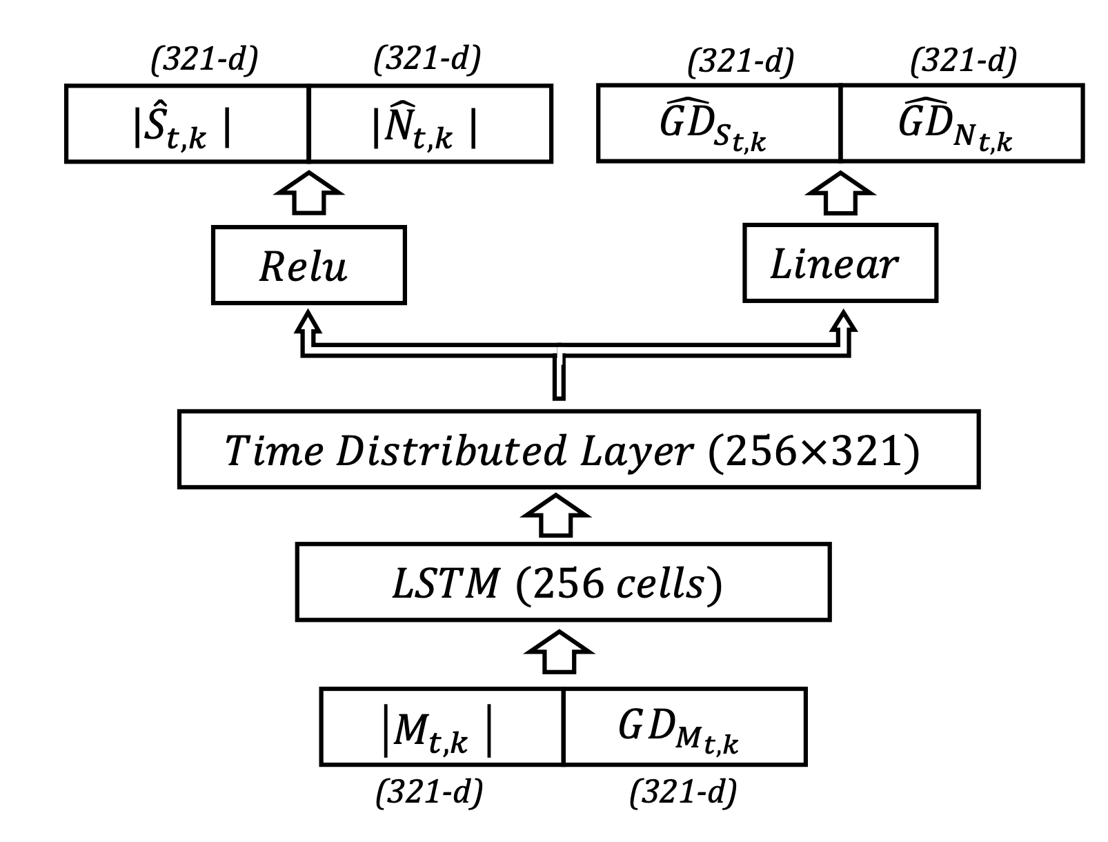
With the above loss function, we train a Baseline LSTM Model. Here, Clean speech and noise are considered as 2 separate sound sources. So each of the signal has their magnitude and phase/group delay. LSTM model takes magnitude of the mixture and the group delay of the mixture as inputs. They are in T-F domain. The output layer is branched in two ways, one is for magnitude approximation, and another is for GD approximation of both speech and noise. Since we have two separate sound sources, Clean speech and noise, there are 4 outputs in total. We use a very naïve deep architecture because our goal is to show the effectiveness from the incorporation of spectral information

Intra-spectral Bi-directional Layer (ISBR)

A time unrolled recurrent network predicts $𝑖^{𝑡ℎ}$ time frame conditioned on the frequency components of the $(𝑖−1)^{𝑡ℎ}$ time frame. From the recurrent network’s point of view, the goal is to capture the temporal influence which is varying over time. Structure or relation across time is learned through this model. Now, Spectral influence can be captured using a frequency unrolled recurrent network. However, this approach is not natural because it uses future frequency points to make the inference. That means to calculate a frequency point of the current time, it infers from the frequency points which are yet to come. In human ears, we sense frequency through the vibration of the basilar membrane, where the root area perceives high frequency and apex area perceives low frequency components. This means human frequency perception is localized and frequencies of the same timestamps are correlated. So this suggests that a frequency component of $𝑖^{𝑡ℎ}$ time depends on its neighbor frequency components of the same time.

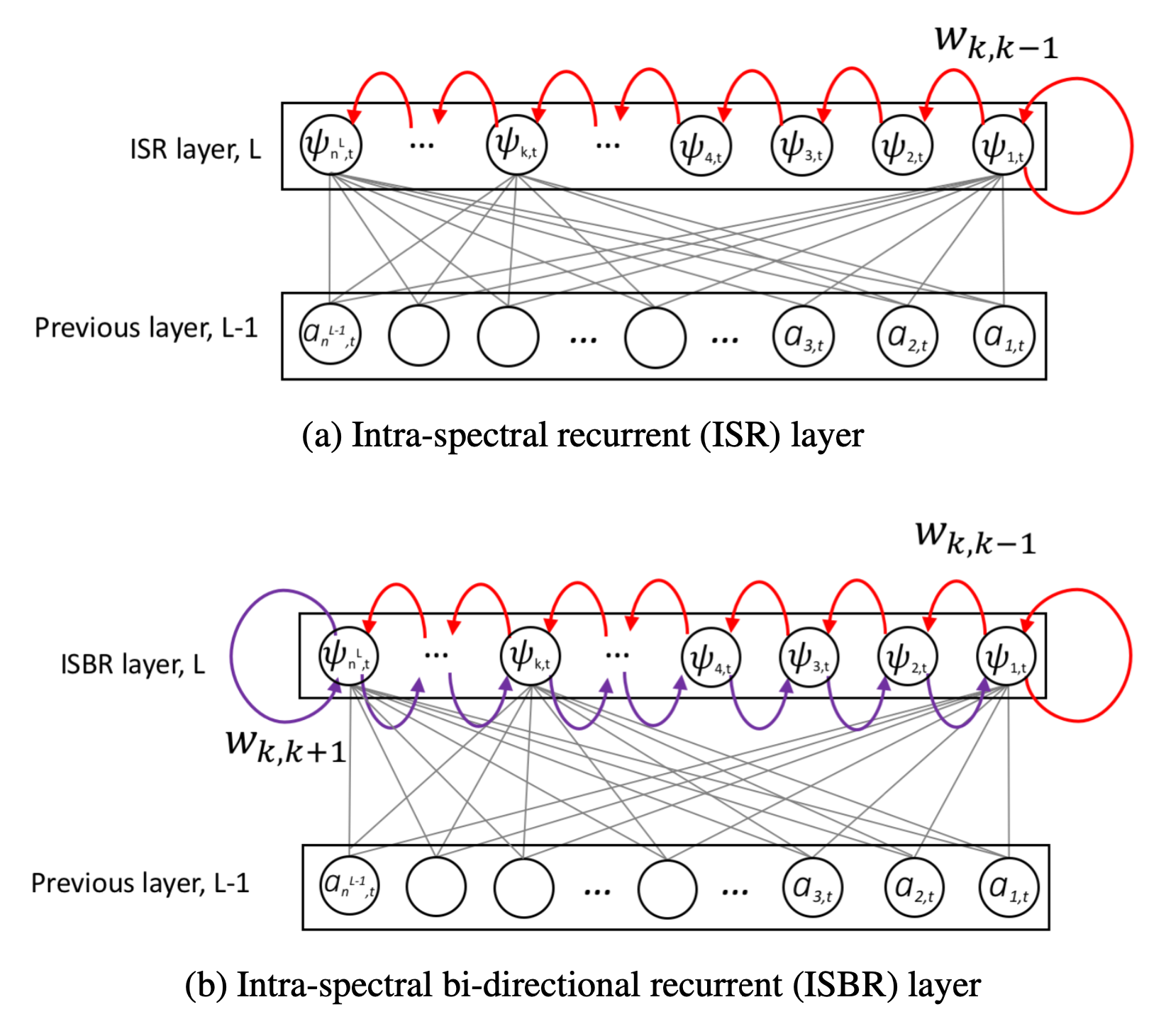
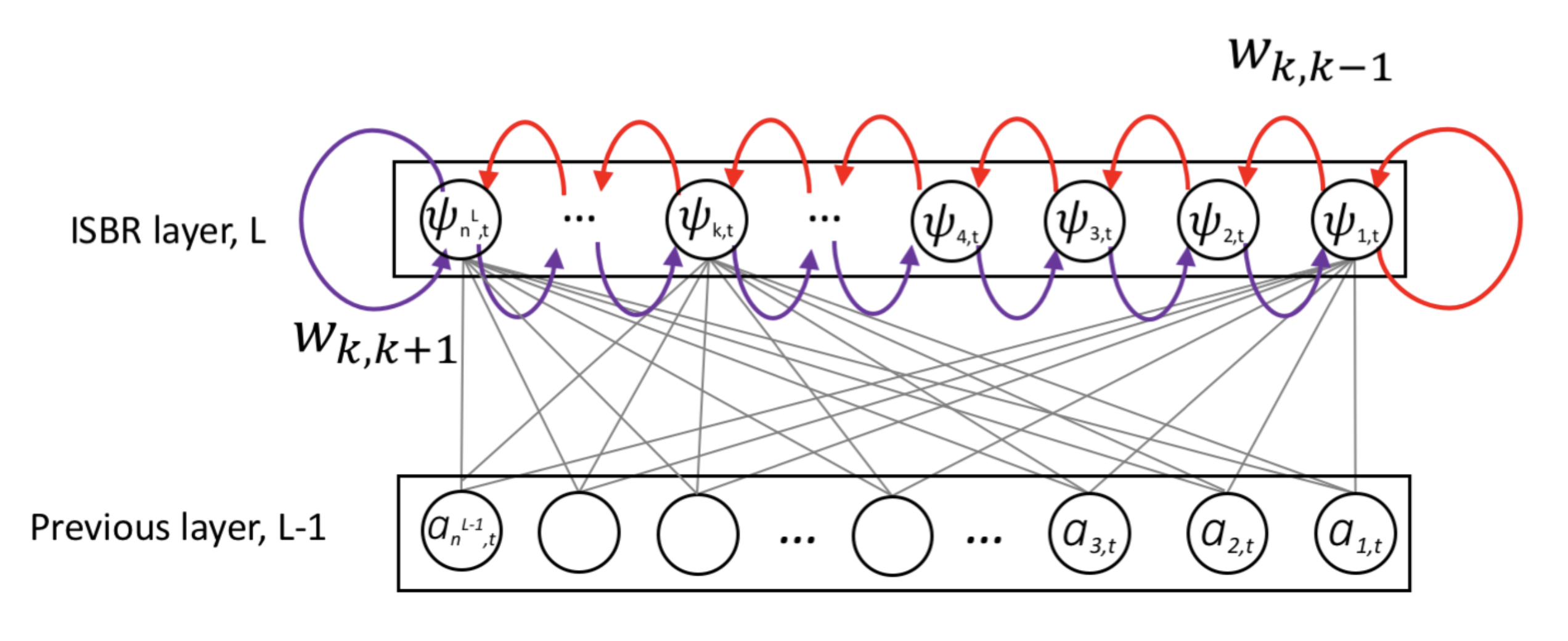
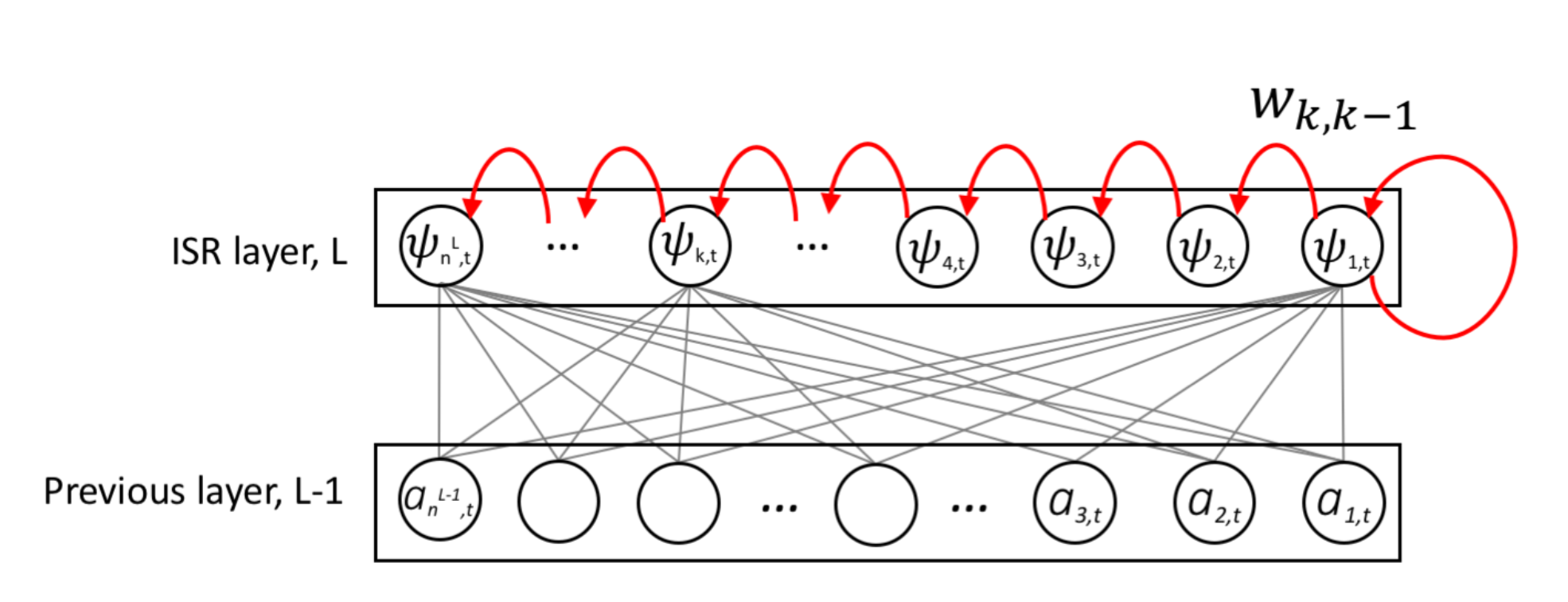
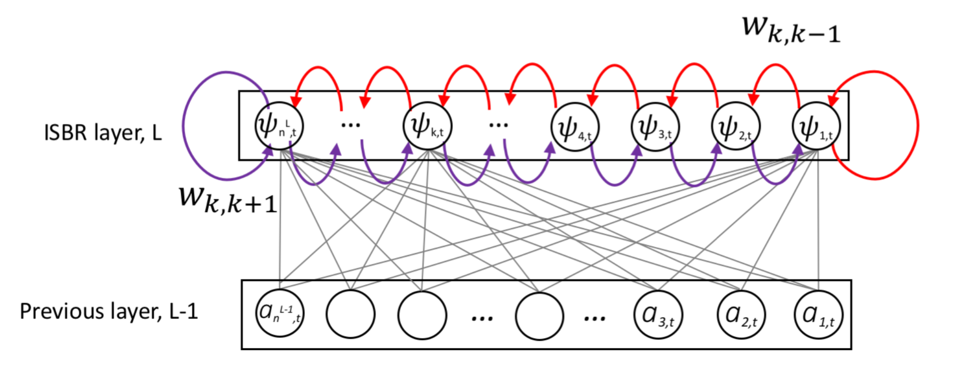
Considering the limitation of regular recurrent layer, we propose Intra-Spectral Bi-directional Recurrent layer (ISBR layer). Each neuron of the ISBR layer represents a frequency bin of the signal. The rightmost neuron represents the lowest frequency component. The leftmost neuron represents the highest frequency component. From left to right, low to high frequencies are modeled and right to left, high to low frequencies are modeled. The intra-spectral recurrences go both (increasing & decreasing) directions along the frequency axis. In the following figure, the red connections represent the increasing or (low to high) frequencies recurrence. And the purple connections represent the decreasing or (high to low) frequencies recurrence.

Results

We compare our proposed approach against 5 other approaches, and the comparison metrics are perceptual evaluation of speech quality (PESQ), short-time objective intelligibility (STOI), scale-invariant signalto-distortion ratio (SI-SDR).

Table 1. Average scores for each approach. Best results are shown in bold.

	IEEE corpus			TIMIT corpus
	PESQ	STOI	SI-SDR	PESQ	STOI	SI-SDR
Mixture	1.86	0.62	-1.47	1.58	0.51	-2.33
L-Stack_mag [1]	2.02	0.59	-0.59	1.82	0.5	-0.84
L-FT_mag [2]	2.05	0.6	-0.2	1.88	0.52	-0.26
L-ISBR_mag [3]	2.24	0.64	0.22	1.93	0.52	-0.03
LSTM_mag+gd	2.24	0.64	0.12	1.97	0.53	-0.1
ISBR_mag+gd	2.34	0.67	0.92	2.04	0.58	0.84
PC-tf-M_mag+phase [4]	2.31	0.67	0.85	2.04	0.58	0.72
PSM_mag+phase [5]	2.27	0.65	0.4	2	0.56	0.32

Our proposed approach outperforms the T-F masking approaches, which indicates that incorporating spectral-level magnitude and phase dependencies are beneficial. We use the ISBR layer with a naïve LSTM approach to show how it can improve the overall performance. Additionally, the proposed ISBR layer can be used as an output layer on top of any state-of-the-art model.

References:

1. J. Deng et al., “Exploiting time-frequency patterns with lstm-rnns for low-bitrate audio restoration,” Neural Computing and Applications, pp. 1–13, 2019.
2. J. Li, A. Mohamed, G. Zweig, and Y. Gong, “LSTM time and frequency recurrence for automatic speech recognition,” in Proc. ASRU, pp. 187–191, 2015.
3. K. M. Nayem and D. S. Williamson, “Incorporating intra-spectral dependencies with a recurrent output layer for improved speech enhancement,” in Proc. MLSP, 2019.
4. J. Lee and H.-G. Kang, “A joint learning algorithm for complex-valued tf masks in deep learning-based single channel speech enhancement systems,” IEEE/ACM TASLP, vol. 27, pp. 1098–1109, 2019.
5. H. Erdogan, J. R. Hershey, S. Watanabe, and J. Le Roux, “Phase-sensitive and recognition-boosted speech separation using deep recurrent neural networks,” in Proc. ICASSP, pp. 708–712, 2015.

×

Incorporating Intra-Spectral Dependencies With A Recurrent Output Layer For Improved Speech Enhancement

For full details, please check out the following paper that is referenced below.

• K. M. Nayem and D. Williamson, "Incorporating intra-spectral dependencies with a recurrent output layer for improved speech enhancement" in IEEE 29th International Workshop on Machine Learning for Signal Processing (MLSP) , pp. 1-6, 2019. [PDF] [POSTER]

Abstract

Deep-learning based speech enhancement systems have offered tremendous gains, where the best performing approaches use long short-term memory (LSTM) recurrent neural networks (RNNs) to model temporal speech correlations. These models, however, do not consider the frequency-level correlations within a single time frame, as spectral dependencies along the frequency axis are often ignored. This results in inaccurate frequency responses that negatively affect perceptual quality and intelligibility. We propose a deep-learning approach that considers temporal and frequency-level dependencies. More specifically, we enforce spectral-level dependencies within each spectral time frame through the introduction of a recurrent output layer that models the Markovian assumption along the frequency axis. We evaluate our approach in a variety of speech and noise environments, and objectively show that this recurrent spectral layer offers performance gains over traditional approaches. We also show that our approach outperforms recent approaches that consider frequency-level dependencies.

Introduction

Speech enhancement, which strives to effectively remove unwanted background noise, is an important problem for several applications, including voice-based home assistants (e.g. Google Home and Amazon Echo), hearing aids, and many military applications. The performance of these devices and applications severely degrades when noise is present, as noise makes it difficult to understand speech, largely due to spectral and temporal masking effects that render the speech inaudible. General deep learning approaches produce T-F outputs that are based on prior network layers and prior (in time) outputs of that T-F unit. In other words, the spectral output at a particular time-frequency point is not based on the spectral output at adjacent or nearby frequency points. This is problematic as it is known that speech has spectral dependencies along the frequency axis. Here we propose an intra-spectral (e.g. across- frequency) recurrent layer that captures frequency dependencies within each time frame of a speech signal. Given a noisy speech input, multiple LSTM layers first capture the temporal dependencies of speech. We then append the proposed intra-spectral recurrent layer to enforce spectral- level dependencies. The entire network is trained to estimate the log-magnitude spectrum of clean speech.

Neutal network-based speech enhancement

Let's define $s_t$ as clean speech and $n_t$ as unwanted noise in time domain. Then $m_t$ denotes noisy speech mixture at time $t$.

$m_t = s_t + n_t $

Using the short-time Fourier transform (STFT), $S_{𝑡,𝑘}$ is the time-frequency (T-F) domain clean speech signal at time $t$ and frequency $k$. Similarly, $M_{t,k}$ is the noisy speech in T-F domain, which is the multiplication of magnitude $|M_{t,k}|$ and exponent of phase $e^{i \theta^M_{t,k}}$.

$M_{t,k} = |M_{t,k}| e^{i \theta_{M_{t,k}}}$

Our aim is to approximate clean speech magnitude $|\hat{𝑆}̂_{𝑡,𝑘}|$ by learning the function $𝐹_\phi$ on noisy mixture magnitude with parameter $\phi$. We reproduce the approximated speech using noisy mixture phase.

$\begin{aligned}|\hat{𝑆}̂_{𝑡,𝑘}| =& 𝐹_\phi(|M_{t,k}|) \\ \hat{𝑆}̂_{𝑡,𝑘} = & |\hat{𝑆}̂_{𝑡,𝑘}| e^{i\theta_{M_{t,k}}}\end{aligned}$

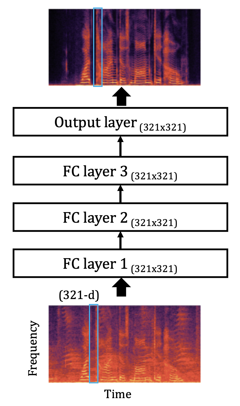
For a baseline, we use a fully connected deep neural network (DNN) where each time frame of $|M_{t,k}|$ is the input and estimated $|\hat{S}_{t,k}|$ is the output. Output of each layer $a^l_t$ is computed by the following equation where $l$ is the layer, $\sigma$ is the activation function, $V^l$ and $z^l$ are weight and bias respectively. However, in a DNN model, outputs are uncorrelated across time and frequency, and spectral output at each neuron does not depend on spectral outputs from other output-layer neurons.

$a^l = \sigma(V^l a^{l-1}_t +z^l)$

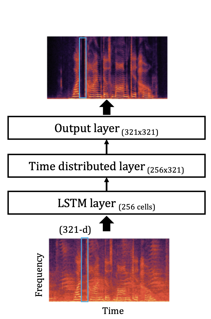
In baseline LSTM, Input and output are magnitude of the spectrogram same as baseline DNN. Output of each layer $a^l_t$ is computed by the following equation where $f^l_t$, $i^l_t$, $o^l_t$ represent $l$-th layer's activation vectors for the forget, input and output gates of a LSTM cell, at time $t$. $h^l$ is the hidden state vector and $c^l_t$ is the cell state vector of the $l$-th layer. Each LSTM layer has $n^l$ LSTM units. Additionally, $W$, $U$, and $b$ are the weight and bias matrices that are optimized during training.

$\begin{aligned} f_t^l &= \sigma_g(W_f^l a_t^{l-1} + U_f^l h^l_{t-1} + b_f^l)\\ i_t^l &= \sigma_g(W_i^l a_t^{l-1} + U_i^l h^l_{t-1} + b_i^l)\\ o_t^l &= \sigma_g(W_o^l a_t^{l-1} + U_o^l h^l_{t-1} + b_o^l)\\ c_t^l &= f_t^l\circ c^l_{t-1}+i^l_t\circ\sigma_c(W_c^l a_t^{l-1} + U_c^l h^l_{t-1} + b^l_c)\\ h_t^l &= o_t^l \circ \sigma_h(c_t^l) \\ a^l_t &= \sigma_a(W_a^l h^l_t + b_a^l) ,\quad l \in [1,L] \end{aligned}$

Intra-spectral Output Layers

To capture intra-spectral correlations with a recurrent layer, we propose to use a first-order Markov assumption. In other words, knowing that adjacent spectral components are dependent, we design a recurrent layer that functions as a Markov chain, where the spectral output at a certain frequency is provided as input to adjacent neurons. This is done along the entire frequency axis. Each neuron in the output layer corresponds to a frequency bin. A traditional LSTM network is first pre-trained, then a ISR/ISBR output layer replaces the original output layer.

Results

We compare our proposed approach against other approaches in different noise conditions, and the comparison metrics are perceptual evaluation of speech quality (PESQ), short-time objective intelligibility (STOI), scale-invariant signalto-distortion ratio (SI-SDR).

Table 1. Average scores of the different models for seen SNRs (e.g. -3, 0 and 3 dB). Best results are shown in bold.

	PESQ				STOI				SI-SDR
	SSN	Cafe	Factory	Babble	SSN	Cafe	Factory	Babble	SSN	Cafe	Factory	Babble
Mixture	1.95	1.86	1.83	1.77	0.71	0.62	0.65	0.59	-0.51	-2.06	-0.96	-1.97
DNN [1]	2.04	1.89	2.02	1.89	0.75	0.63	0.72	0.56	-1.75	-1.1	-1.4	-1.39
LSTM	2.12	1.97	2.05	1.95	0.77	0.64	0.76	0.62	-0.96	-1.35	-0.15	-0.44
D-ISR	2.24	2.08	2.26	2.08	0.85	0.76	0.86	0.76	-1.49	-2.91	-2.75	-3.48
L-ISR	2.27	2.21	2.29	2.11	0.82	0.68	0.84	0.72	0.06	-1.34	0.17	-1.3
L-ISBR	2.3	2.24	2.31	2.13	0.88	0.74	0.87	0.73	2.35	-0.12	-0.94	-0.01
L-FT [2]	2.12	2.01	2.07	2.04	0.82	0.74	0.82	0.66	1.04	-1.16	-0.88	-0.1

We compare the STOI and SI_SDR scores in different signal-to-noise ratio (SNR). In terms of SI-SDR, our proposed L-ISBR approach performs best at each SNR, where it performs noticeably better at the more challenging lower SNR cases. According to STOI, the D-ISR and L-ISBR approaches perform similarly at most SNRs, and best overal.

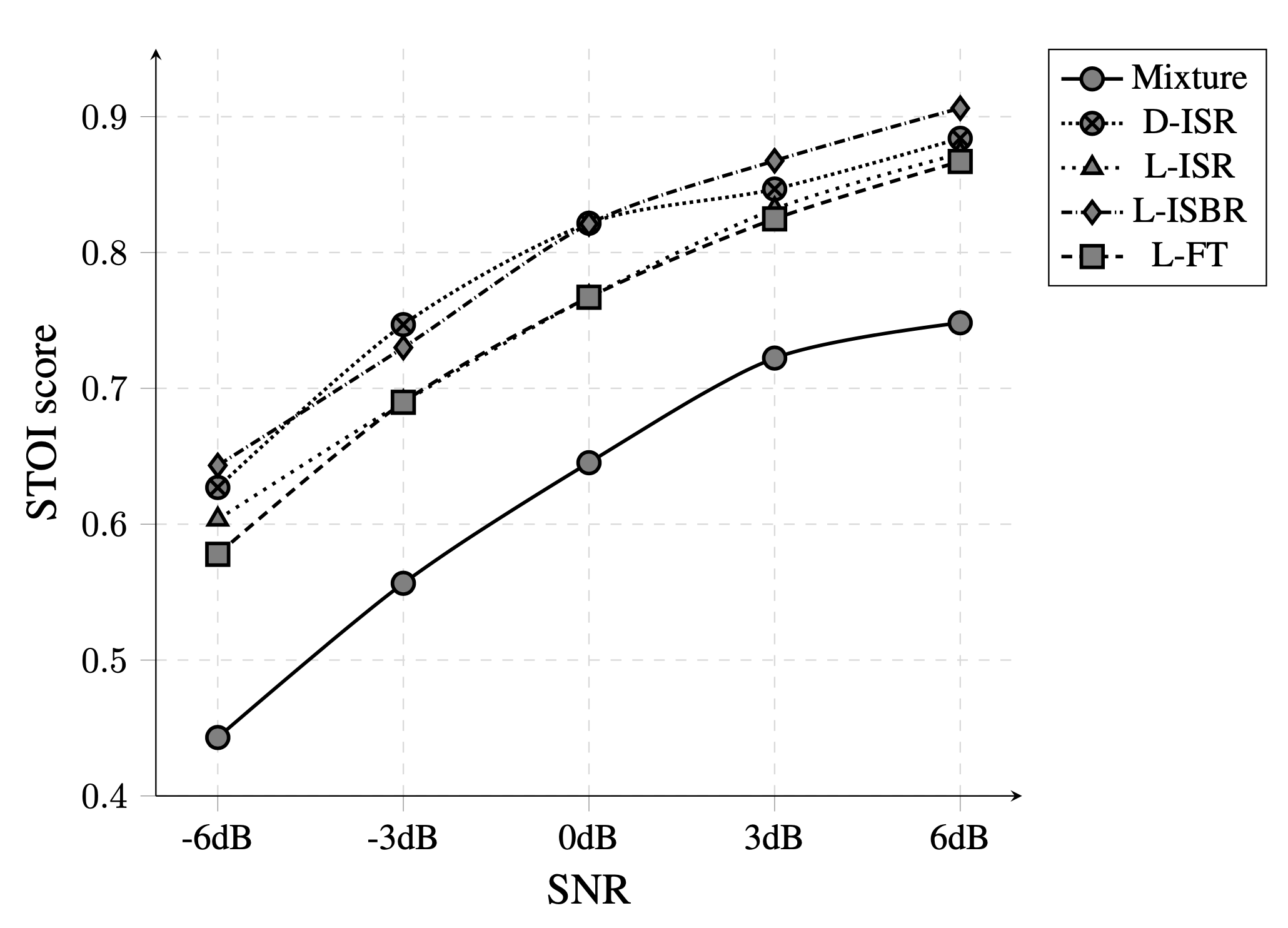
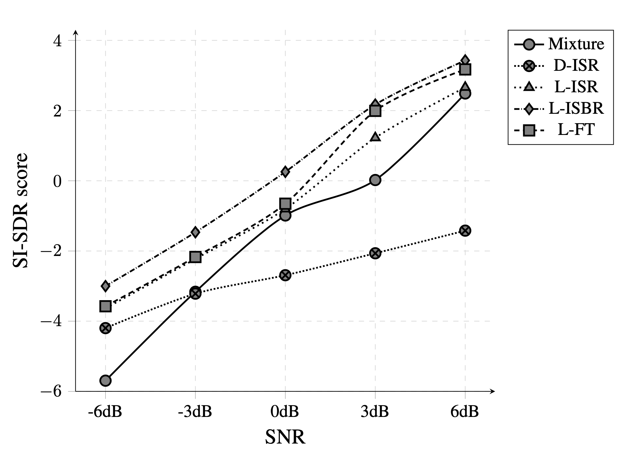
Improvements in a variety of noises and SNR values prove that the proposed ISR/ISBR layer along with a base LSTM network successfully captures both temporal and spectral correlations. Additionally, overall performace of LSTM network with ISR/ISBR layer (L-ISR/L-ISBR) shows the correlation between adjacent frequencies are important in the estimation of clean speech.

References:

1. Y. Xu, J. Du, L.-R. Dai, and C.-H. Lee, “A regression approach to speech enhancement based on deep neural networks,” in Proc. IEEE/ACM Transactions on Audio, Speech and Language Processing (TASLP), pp 7-19, 2015.
2. J. Li, A. Mohamed, G. Zweig, and Y. Gong, “LSTM time and frequency recurrence for automatic speech recognition,” in Proc. ASRU, pp. 187–191, 2015.

×

Impact of Amplification on Speech Enhancement Algorithms

Please refer to the paper below for full details about the effects of speech amplification on the hearing-impaired population.

• Z. Zhang, D. Williamson, and Y. Shen, "Impact of Amplification on Speech Enhancement Algorithms Using an Objective Evaluation Metric," Proc. International Congress on Acoustics (ICA), 2019. [PDF]

Abstract

Hearing loss is prevalent among elderly adults, which leads to speech-understanding difficulties in noisy environments. Speech enhancement algorithms are thus proposed to alleviate this speech-in-noise problem. However, most of these algorithms have not been evaluated for hearing-impaired people either with or without the use of hearing aids. In this study, we evaluated the performance of several speech enhancement algorithms [i.e., nonnegative matrix factorization based, deep-neural-network based and long short-term memory (LSTM) based algorithms] for hearing-impaired listeners using an objective speech quality metric, namely the Hearing-Aid Speech Quality Index (HASQI). The HASQI is based on a physiologically inspired model of auditory processing, which also allows the simulation of hearing impairment. The evaluation was repeated separately for the typical hearing characteristics of different genders in various age groups. For the aided condition, linear amplification was implemented using the NAL-R prescription formula. The benefits from the speech enhancement algorithms decrease with increasing degrees of hearing loss. With amplification, the benefit diminishes for the listener group with the most severe hearing impairment. Among the various algorithms, the LSTM-based structures exhibit superior performance with and without amplification.

Introduction

The goal of speech enhancement algorithms is to remove the undesired noise from the noisy speech. It is hypothesized that applying amplification to the enhanced speech signals would improve speech understanding for listeners with age-related hearing loss. This study investigates the perceived speech quality following speech enhancement and amplification from hearing-impaired listeners using an objective speech-quality metric, HASQI [1]. In our previous work [2], no compensation for the loss of audibility was applied for the hearing-impaired groups, therefore, it is possible that the decreased HASQI scores merely reflected the reduced available speech bandwidth due to hearing loss. In the current study, the evaluations conducted by Zhang et al. [2] are repeated with and without amplification applied following speech enhancement.

Speech Enhancement Algorithms

1. Active-set Newton algorithm [3]:
As an extension of NMF, the active-set Newton algorithm (ASNA) is expressed as $\hat{x} = Bw$, where $\hat{x}$ is the target speech signal, $B$ is the trained speech dictionary and $w$ represents the activation weights. This approach applies the Newton method to update the weights more efficiently than other NMF approaches.

2. DNN-based ideal ratio mask estimation [4]:
The network has three hidden layers with 1024 units each. ReLU activation function is applied to the hidden layers and a linear activation function is applied to the output layer. A set of complementary features [4] are used as the input to the network. The ideal ratio mask (IRM) is used as the training target, which is defined as: $M_{t,f}^{rm}=\left|s_{t,f}\right|/(\left|s_{t,f}\right|+\left|n_{t,f}\right|)$. The mean-squared error (MSE) loss function is used for training. This approach is denoted as D-IRM.

3. DNN-based complex ideal ratio mask estimation [5]:
The network consists of three hidden layers with 1024 units each. All hidden layers use ReLU activation functions. The output layer uses a linear activation function. The complex ideal ratio mask (cIRM) can be defined as: $M_{t,f}^{crm}=\frac{\left|s_{t,f}\right|}{\left|y_{t,f}\right|}\cos(\theta_{t,f})+j\frac{\left|s_{t,f}\right|}{\left|y_{t,f}\right|}\sin(\theta_{t,f})$, where $\left|y_{t,f}\right|$ represents the magnitude response of the noisy speech, $j$ indicates a imaginary number, and $\theta_{t,f} = \theta^s_{t,f}-\theta^y_{t,f} $, e.g., the phase difference between the speech and noisy speech. The mean-squared error (MSE) loss function is used for training. This approach is denoted as D-cIRM.

4. LSTM-based ideal ratio mask estimation [6]:
The network has two LSTM layers with 256 nodes in each layer, followed by a third sigmoidal layer with 257 units. IRM is used as the target mask.
Mask approximation (MA) [6] is adopted as the loss function: $E^{MA}\left(M_{pred}\right)=\sum_{t,f}{(M_{true}-M_{pred})}^2 $, where $M_{pred}$ is the predicted mask and $M_{true}$ is the IRM. This approach is denoted as L-IRM.

5. Bidirectional LSTM-based Phase-sensitive Mask estimation [7]:
A similar network structure to the LSTM network, two layers of Bi-LSTM (256 nodes each) and another layer of fully connected neurons with 257 units. The phase-sensitive mask (PSM) is used as target, defined as $M_{t,f}^{psm} = \frac{|s_{t,f}|}{|y_{t,f}| }cos(\theta_{t,f})$. A phase-sensitive spectrum approximation (PSA) is used as the cost function: $E^{PSA}\left(M_{pred}\right)=\sum_{t,f}{(M_{true}|y_{t,f}|-M_{pred}|y_{t,f}|)}^2$, where $M_{true}$ is the ideal PSM and $M_{pred}$ is the estimated one. This approach is denoted as BL-PSM.

Hearing Thresholds

HASQI requires the auditory thresholds as input to simulate hearing loss. Below is the auditory thresholds we collected from [8].

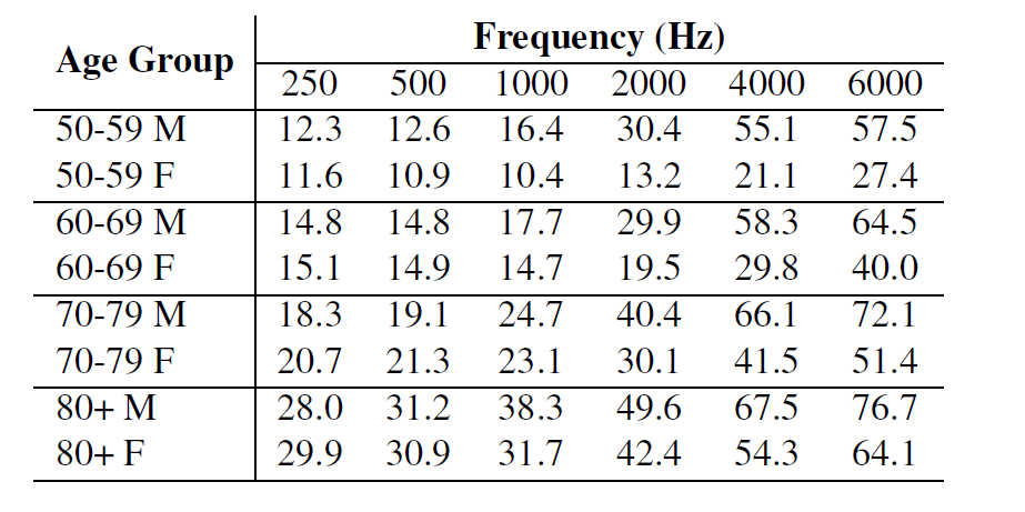
Hearing thresholds (dB HL) of male (M) and female (F) subjects across different age groups.

Speech Materials

Utterances from three speech corpora are combined, in order to investigate the performance of the above-described algorithms on diverse speech materials. The speech data includes 1440 IEEE utterances for both male and female speakers, 250 male-speech utterances from the Hearing in Noise Test (HINT) corpus and 2342 male and female utterances from the TIMIT database. The clean utterances are further corrupted by four types of noises at different levels, including airplane, babble, dog barking, and train noises. The clean speech and noise are mixed at several SNRs ranging from -5 dB to 20 dB with a step of 5 dB. All signals are resampled at 16 kHz.

Linear Amplification

In the current study, the clean reference signal is amplified according to a standard hearing-aid prescription formula (i.e. NAL-R) [9]. This formula generates a fixed gain, independent of input level (i.e. linear amplification), for each of the frequency regions. Therefore, the reference signal used for computing the HASQI score represents speech heard in quiet through typical linear amplification.

For each combination of speech enhancement algorithm and listener group, speech quality is calculated using HASQI either before (“Mixture") or after (“Enhanced") speech enhancement is applied, and with (“Eq. On") or without (“Eq. Off") amplification. The test signal that is used to calculate the HASQI score is different depending on the condition. Specifically, when no amplification is applied, the noisy speech mixture is used in the “Mixture Eq. Off" condition, and the enhanced speech is used in the “Enhanced Eq. Off" condition. When amplification is applied, the test signal is the the noisy speech mixture amplified according to the NAL-R formula in the “Mixture Eq. On" condition, and it is the enhanced speech amplified according to the NAL-R formula in the “Enhanced Eq. On" condition.

Experimental Results

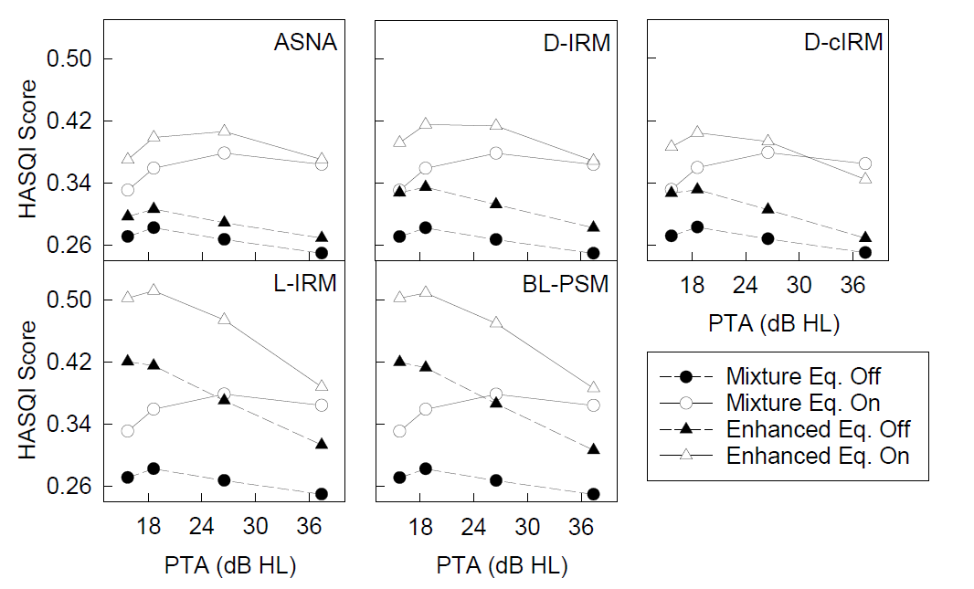
HASQI (from 0 to 1) results with NAL-R amplification on and off. Each curve in a panel shows the HASQI score as a function of pure-tone-average (PTA) threshold, which is the average of the thresholds at 500, 1000, and 2000 Hz (i.e., frequencies that are most important for speech understanding). The four data points along each curve indicate the four listener groups, the group with a higher age range corresponds to a higher PTA threshold.

As shown in the figure above, amplification always leads to improvement in speech quality. Without speech enhancement, the benefit from amplification increases slightly as the degree of hearing loss increases (comparing filled and unfilled circles). This effect of hearing loss is less evident when speech enhancement is applied. Across all five speech enhancement algorithms, speech enhancement improved the predicted speech quality by HASQI (comparing triangles to circles). However, under the conditions with amplification, the benefit from speech enhancement diminishes as the PTA threshold increases. The LSTM- and BLSTM-based structure perform the best among the algorithms both with and without amplification. We infer that as the degree of hearing loss increases, there will be fewer benefits from wearing a digital hearing aid device with built-in speech enhancement.

References:

• [1]. J. M. Kates and K. H. Arehart, “The hearing-aid speech quality index (HASQI) version 2,” Journal of the Audio Engineering Society, vol. 62, pp. 99–117, 2014.
• [2]. Z. Zhang, Y. Shen, and D. S. Williamson, “Objective comparison of speech enhancement algorithms with hearing loss simulation,” in ICASSP 2019-2019 IEEE International Conference on Acoustics, Speech and Signal Processing (ICASSP). IEEE, 2019, pp. 6845–6849.
• [3]. T. Virtanen, J. F. Gemmeke, and B. Raj, “Active-set newton algorithm for overcomplete non-negative representations of audio,” IEEE Trans. ASSP, vol. 21, pp. 2277–2289, 2013.
• [4]. Y. Wang, A. Narayanan, and D. L. Wang, “On training targets for supervised speech separation,” TASLP, vol. 22, pp. 1849–1858, 2014.
• [5]. D. Williamson, Y. Wang, and D. L. Wang, “Complex ratio masking for monaural speech separation,” TASLP, vol. 24, pp. 483–492, 2016.
• [6]. F. Weninger, J. R. Hershey, J. Le Roux, and B. Schuller, “Discriminatively trained recurrent neural networks for single-channel speech separation,” in Proc. GlobalSIP, 2014.
• [7]. H. Erdogan, J. R. Hershey, S.Watanabe, and J. Le Roux, “Phase-sensitive and recognition-boosted speech separation using deep recurrent neural networks,” in Proc. ICASSP, 2015, pp. 708–712.
• [8]. R. A. Schmiedt, “The physiology of cochlear presbycusis,” in The aging auditory system, pp. 9–38. 2010.
• [9]. D. Byrne and H. Dillon, “The national acoustic laboratories’(nal) new procedure for selecting the gain and frequency response of a hearing aid,” Ear and hearing, vol. 7, no. 4, pp. 257–265, 1986.

×

Evaluation of Speech Enhancement Algorithms with Simulated Hearing Loss

Please refer to the paper below for full details.

• Z. Zhang, Y. Shen, and D. Williamson, "Objective Comparison of Speech Enhancement Algorithms with Hearing Loss Simulation," Proc. IEEE International Conference on Acoustics, Speech, and Signal Processing (ICASSP), pp 6845-6849, 2019. [PDF]

Abstract

Many speech enhancement algorithms have been proposed over the years and it has been shown that deep neural networks can lead to significant improvements. These algorithms, however, have not been validated for hearing-impaired listeners. Additionally, these algorithms are often evaluated under a limited range of signal-to-noise ratios (SNR). Here, we construct a diverse speech dataset with a broad range of SNRs and noises. Several enhancement algorithms are compared under both normal-hearing and simulated hearingimpaired conditions, where the perceptual evaluation of speech quality (PESQ) and hearing-aid speech quality index (HASQI) are used as objective metrics. The impact of the data's frequency scale (Mel versus linear) on performance is also evaluated. Results show that a long short-term memory (LSTM) network with data in the Mel-frequency domain yields the best performance for PESQ, and a Bidirectional LSTM network with data in the linear frequency scale performs the best in hearing-impaired settings. The Mel-frequency scale results in improved PESQ scores, but reduced HASQI scores.

Introduction

Speech degradation in the presence of noise is a common problem for individuals, especially for people with hearing impairments. Yet many speech enhancement algorithms have not been validated for hearing-impaired listeners. In this study, we mainly investigate 5 different speech enhancement algorithms [1,2,3,4,5] and evaluate their effectiveness in simulated hearing-impaired listeners by using HASQI [6] as one of the evaluation metric. Meanwhile, the impact of the frequency scale (Mel versus linear) is also investigated, since studies have used different frequency scales without performing direct comparisons. PESQ is also included as the other evaluation metric.

Speech Enhancement Algorithms

1. Active-set Newton algorithm [1]:
As an extension of NMF, the active-set Newton algorithm (ASNA) is expressed as
$\hat{x} = Bw$
where $\hat{x}$ is the target speech signal, $B$ is the trained speech dictionary and $w$ represents the activation weights. This approach applies the Newton method to update the weights more efficiently than other NMF approaches.

2. DNN-based ideal ratio mask estimation [2]:
The network has three hidden layers with 1024 units each. ReLU activation function is applied to the hidden layers and a linear activation function is applied to the output layer. A set of complementary features [2] are used as the input to the network. The ideal ratio mask (IRM) is used as the training target, which is defined as:
$M_{t,f}^{rm}=\left|s_{t,f}\right|/(\left|s_{t,f}\right|+\left|n_{t,f}\right|)$
For all deep learning based systems, we implement them in both the linear and Mel frequency domain, where the transformation between Mel and linear scale is defined as:
$|s_{t,f}^{Mel}| = B|s_{t,f}|, \quad |s_{t,f}^{iMel}| = B^{T}|s_{t,f}^{Mel}|$
where ${|s}_{t,f}^{Mel}|$ is the Mel-domain signal and $|s_{t,f}^{iMel}|$ is the linear scale signal after an inverse-Mel transformation. $B$ represents a matrix of weights to combine short-time Fourier transform (STFT) bins into Mel bins, and $B^{T}$ represents the transpose of $B$. Note that Mel-transformation is a lossy process.
Loss function: Mean squared error.
This approach is denoted as D-IRM.

3. DNN-based complex ideal ratio mask estimation [3]:
The network consists of three hidden layers with 1024 units each. All hidden layers use ReLU activation functions. The output layer uses a linear activation function. The complex ideal ratio mask (cIRM) can be defined as:
$M_{t,f}^{crm}=\frac{\left|s_{t,f}\right|}{\left|y_{t,f}\right|}\cos(\theta_{t,f})+j\frac{\left|s_{t,f}\right|}{\left|y_{t,f}\right|}\sin(\theta_{t,f})$
where $\left|y_{t,f}\right|$ represents the magnitude response of the noisy speech, $j$ indicates a imaginary number, and $\theta_{t,f} = \theta^s_{t,f}-\theta^y_{t,f} $, e.g., the phase difference between the speech and noisy speech.
Loss function: Mean squared error.
This approach is denoted as D-cIRM.

4. LSTM-based ideal ratio mask estimation [4]:
The network has two LSTM layers with 256 nodes in each layer, followed by a third sigmoidal layer. IRM is used as the target mask.
Mask approximation (MA) [4] is adopted as the loss function:
$E^{MA}\left(M_{pred}\right)=\sum_{t,f}{(M_{true}-M_{pred})}^2 $
where $M_{pred}$ is the predicted mask and $M_{true}$ is the IRM.
This approach is denoted as L-IRM.

5. Bidirectional LSTM-based Phase-sensitive Mask estimation [5]:
A similar network structure to the LSTM network, two layers of Bi-LSTM (256 nodes each) and another layer of fully connected neurons. The phase-sensitive mask (PSM) is used as target, defined as
$M_{t,f}^{psm} = \frac{|s_{t,f}|}{|y_{t,f}| }cos(\theta_{t,f})$
A phase-sensitive spectrum approximation (PSA) is used as the cost function:
$E^{PSA}\left(M_{pred}\right)=\sum_{t,f}{(M_{true}|y_{t,f}|-M_{pred}|y_{t,f}|)}^2$
where $M_{true}$ is the ideal PSM and $M_{pred}$ is the estimated one.
This approach is denoted as BL-PSM.

Hearing Thresholds

HASQI requires the auditory thresholds as input to simulate hearing loss. Below is the auditory thresholds we collected from [7].

Hearing thresholds (dB HL) of male (M) and female (F) subjects across different age groups.

Speech Materials

Utterances from three speech corpora are combined, in order to investigate the performance of the above-described algorithms on diverse speech materials. The speech data includes 1440 IEEE utterances for both male and female speakers, 250 male-speech utterances from the Hearing in Noise Test (HINT) corpus and 2342 male and female utterances from the TIMIT database. The clean utterances are further corrupted by four types of noises at different levels, including airplane, babble, dog barking, and train noises. The clean speech and noise are mixed at several SNRs ranging from -5 dB to 20 dB with a step of 5 dB.

Simulation Results

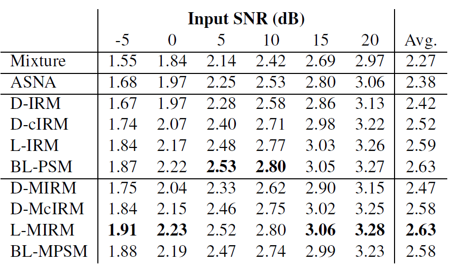
(From left to right) PESQ (from -0.5 to 4.5) results, HASQI (from 0 to 1) results. The D-MIRM, D-McIRM, L-MIRM, and BL-MPSM represent the corresponding systems that are implemented in the Mel frequency domain.

The RNN-based methods result in significantly higher PESQ and HASQI scores for normal-hearing listeners. For hearingimpaired listeners, the BLSTM method achieves the best performance in all age groups for both genders. We also found that for both DNN- and RNN-based methods, Mel-frequency domain processing can often lead to improved PESQ scores, but reduced HASQI scores.

References:

• [1]. T. Virtanen, J. F. Gemmeke, and B. Raj, “Active-set newton algorithm for overcomplete non-negative representations of audio,” IEEE Trans. ASSP, vol. 21, pp. 2277–2289, 2013.
• [2]. Y. Wang, A. Narayanan, and D. L. Wang, “On training targets for supervised speech separation,” TASLP, vol. 22, pp. 1849–1858, 2014.
• [3]. D. Williamson, Y. Wang, and D. L. Wang, “Complex ratio masking for monaural speech separation,” TASLP, vol. 24, pp. 483–492, 2016.
• [4]. F. Weninger, J. R. Hershey, J. Le Roux, and B. Schuller, “Discriminatively trained recurrent neural networks for single-channel speech separation,” in Proc. GlobalSIP, 2014.
• [5]. H. Erdogan, J. R. Hershey, S.Watanabe, and J. Le Roux, “Phase-sensitive and recognition-boosted speech separation using deep recurrent neural networks,” in Proc. ICASSP, 2015, pp. 708–712.
• [6]. J. M. Kates and K. H. Arehart, “The hearing-aid speech quality index (HASQI) version 2,” Journal of the Audio Engineering Society, vol. 62, pp. 99–117, 2014.
• [7]. R. A. Schmiedt, “The physiology of cochlear presbycusis,” in The aging auditory system, pp. 9–38. 2010.

×

GAN-based Speech Enhancement

For full details, please refer to the paper listed below.

• Z. Zhang, C. Deng, Y. Shen, D. Williamson, Y. Sha, Y. Zhang, H. Song, and X. Li, "On Loss Functions and Recurrency Training for GAN-based Speech Enhancement Systems," accepted by ISCA INTERSPEECH, 2020. [PDF]

Abstract

Recent work has shown that it is feasible to use generative adversarial networks (GANs) for speech enhancement, however, these approaches have not been compared to state-of-the-art (SOTA) non GAN-based approaches. Additionally, many loss functions have been proposed for GAN-based approaches, but they have not been adequately compared. In this study, we propose novel convolutional recurrent GAN (CRGAN) architectures for speech enhancement. Multiple loss functions are adopted to enable direct comparisons to other GAN-based systems. The benefits of including recurrent layers are also explored. Our results show that the proposed CRGAN model outperforms the SOTA GAN-based models using the same loss functions and it outperforms other non-GAN based systems, indicating the benefits of using a GAN for speech enhancement. Overall, the CRGAN model that combines an objective metric loss function with the mean squared error (MSE) provides the best performance over comparison approaches across many evaluation metrics.

Introduction

Generative adversarial networks (GANs) was initially proposed to estimating the generative model in the image genearation field. More recently, it has been applied to speech enhancement field where the generator is used to predict the clean speech or clean speech mask, and the discriminator serves as the adversarial component that estimates the probability of samples coming from the training data [1].

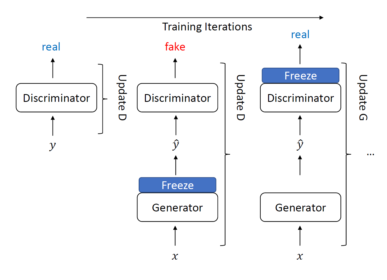
During adversarial training, G will learn a mapping from X to Y. A depiction of the GAN-based training procedure is shown in the figure below. The discriminator D and generator G are trained alternately.

Network Structure

Convolutional Recurrent GAN (CRGAN) structure. The generator estimates a T-F mask. The arrows between layers represent skip connections. The target T-F mask and estimated mask are provided as inputs to the discriminator for all proposed models except W-CRGAN.

Evaluated Loss Functions

Several different loss functions are evaluated for GAN-based speech enhancement systems, including:

• 1. Wasserstein Loss [2]:
  

  \begin{aligned} \mathcal{L}_{D} &= -\mathbb{E}_{y \sim \mathcal{Y}}[D_l(y)] + \mathbb{E}_{x \sim \mathcal{X}}[D_l(G(x))]\\ \mathcal{L}_{G} &=-\mathbb{E}_{x \sim \mathcal{X}}[D_l(G(x))] \end{aligned}

• 2. Relativistic Loss Loss [3]:
  

  \begin{aligned} \mathcal{L}_{D} &=-\mathbb{E}_{(x, y) \sim(\mathcal{X}, \mathcal{Y})}[\log (\sigma(D_l(y)-D_l(G(x))))] \\ \mathcal{L}_{G} &=-\mathbb{E}_{(x, y) \sim(\mathcal{X}, \mathcal{Y})}[\log (\sigma(D_l(G(x))-D_l(y)))] \end{aligned}

• 3. Relativistic average Loss Loss [3]:
  

  \begin{aligned} \mathcal{L}_{D} &=-\mathbb{E}_{y \sim \mathcal{Y}}[\log (\overline{D}_{y})]-\mathbb{E}_{x \sim \mathcal{X}}[\log (1-\overline{D}_{G(x)})] \\ \mathcal{L}_{G} &=-\mathbb{E}_{x \sim \mathcal{X}}[\log (\overline{D}_{G(x)})]-\mathbb{E}_{y \sim \mathcal{Y}}[\log (1-\overline{D}_{y})] \end{aligned}

• 4. Metric Loss [4]:
  

  \begin{aligned} \mathcal{L}_{D} &=\mathbb{E}_{(x, s) \sim(\mathcal{X}, \mathcal{S})}[(D_l(s, s)-1)^{2}\\ & + (D_l(G(x), s)-Q^{\prime}(iSTFT(G(x)), iSTFT(s)))^{2}] \\ \mathcal{L}_{G} &=\mathbb{E}_{x \sim \mathcal{X}}[(D_l(G(x), s)-1)^{2}] \end{aligned}

Experimental Results

Results for the enhancement systems (W-CRGAN, R-CRGAN, Ra-CRGAN and M-CRGAN denote our proposed CRGAN models with Wasserstein, relativisitc, relativisitc average and metric losses, respectively.) Best scores are highlighted in bold. (* indicates previously reported results.)

References:

• [1]. Goodfellow, I., Pouget-Abadie, J., Mirza, M., Xu, B., Warde-Farley, D., Ozair, S., Courville, A. and Bengio, Y., 2014. Generative adversarial nets. In Advances in neural information processing systems (pp. 2672-2680).
• [2]. M. Arjovsky, S. Chintala, and L. Bottou, “Wasserstein gan,” arXiv preprint arXiv:1701.07875, 2017.
• [3]. A. Jolicoeur-Martineau, “The relativistic discriminator: a key element missing from standard gan,” arXiv preprint arXiv:1807.00734, 2018.
• [4]. S. W. Fu, C. F. Liao, Y. Tsao, and S. D. Lin, “Metricgan: Generative adversarial networks based black-box metric scores optimization for speech enhancement,” arXiv preprint arXiv:1905.04874, 2019.

×

Influence of Phase Distortions on Hearing-impaired Listeners

For full details, please refer to the paper listed below.

• Z. Zhang, D. Williamson, and Y. Shen, "Investigation of Phase Distortion on Perceived Speech Quality for Hearing-impaired Listeners," ISCA INTERSPEECH, 2020. [PDF]

Abstract

Phase serves as a critical component of speech that influences the quality and intelligibility. Current speech enhancement algorithms are beginning to address phase distortions, but the algorithms focus on normal-hearing (NH) listeners. It is not clear whether phase enhancement is beneficial for hearing-impaired (HI) listeners. We investigated the influence of phase distortion on speech quality through a listening study, in which NH and HI listeners provided speech-quality ratings using the MUSHRA procedure. In one set of conditions, the speech was mixed with babble noise at 4 different signal-to-noise ratios (SNRs) from -5 to 10 dB. In another set of conditions, the SNR was fixed at 10 dB and the noisy speech was presented in a simulated reverberant room with T60s ranging from 100 to 1000 ms. The speech level was kept at 65 dB SPL for NH listeners and amplification was applied for HI listeners to ensure audibility. Ideal ratio masking (IRM) was used to simulate speech enhancement. Two objective metrics (i.e., PESQ and HASQI) were utilized to compare subjective and objective ratings. Results indicate that phase distortion has a negative impact on perceived quality for both groups and PESQ is more closely correlated with human ratings.

Introduction

Many of the existing speech enhancement systems only operate based on the magnitude spectrogram and keep the noisy phase unchanged when converting the enhanced speech to the time domain [1,2]. Phase is important for speech but has been studied less commonly, studies that focused on recovering phase information for enhancement algorithms only focused on normal-hearing listeners. However, there is a large number of people who are suffered from hearing loss which can degrade their sensitivity to temporal fine structure (TFS) cues. Therefore, it may be expected that preserving the phase information in speech enhancement may not lead to the same degree of benefit for HI listeners compared to NH listeners. In this study, we investigate whether hearing-impaired listeners would benefit from a phase-aware speech enhancement system and analyze the correlation between subjective scores and objective scores from HASQI and PESQ.

Phase Distortion

Different degrees of phase distortion is applied to the speech material (IEEE sentences from a female talker) according to the formula:

$\angle s(t,f)_{\text{distorted}} = \angle s(t,f) + \alpha \cdot \phi(t,f)$

where $\angle s(t,f)_{\text{distorted}}$ denotes the distorted phase in the T-F domain; $\alpha$ denotes the amount of phase distortion ranging from 25% to 100%; and $\phi(t,f)$ represents random phase perturbations drawn from a uniform distribution between 0 and $2\pi$, independently for each T-F location.

Listening Study

Listeners provided subjective ratings on the stimuli following the MUSHRA procedure, recommended in ITU-R BS.1534 [3]
A total of 18 participants were recruited, including 10 NH listeners (4 males, 6 females, recruited from the undergraduate population at Indiana University) and 8 HI listeners (3 males, 5 females, average age: 68 ($SD = 5.53$)).

There were four test conditions in the listening test. In the Noisy condition, the speech stimuli was presented with babble noise at 4 different signal-to-noise ratios (SNRs), from -5 dB to 10 dB with a 5 dB step. In the Noisy-Enhanced condition, the stimuli were the same as those in the Noisy condition except that they were further masked by the ideal ratio mask (IRM) [1] before presentation. In the Reverberant condition, the SNR between the speech and noise was fixed at 10 dB and the stimuli were presented with simulated reverberation [4]. The reverberation algorithm simulated a room with a dimension of 4m$\times$4m$\times$3m (length$\times$width$\times$height), the sound source was located at (2m, 3.5m, 2m), and the listener was located at (2m, 1.5m, 2m). The sound velocity was assumed to be 340 m/s. The reverberation times (T60) were 100, 200, 500, and 1000 ms. In the Reverbrant-Enhanced condition, the stimuli were the same as those in the Reverbrant condition except that they were further masked by the IRM before presentation. Note that the IRM in this condition was applied only on the noise without removing reverberation, which resembles a system that is not trained on reverberant data.

Experimental Results

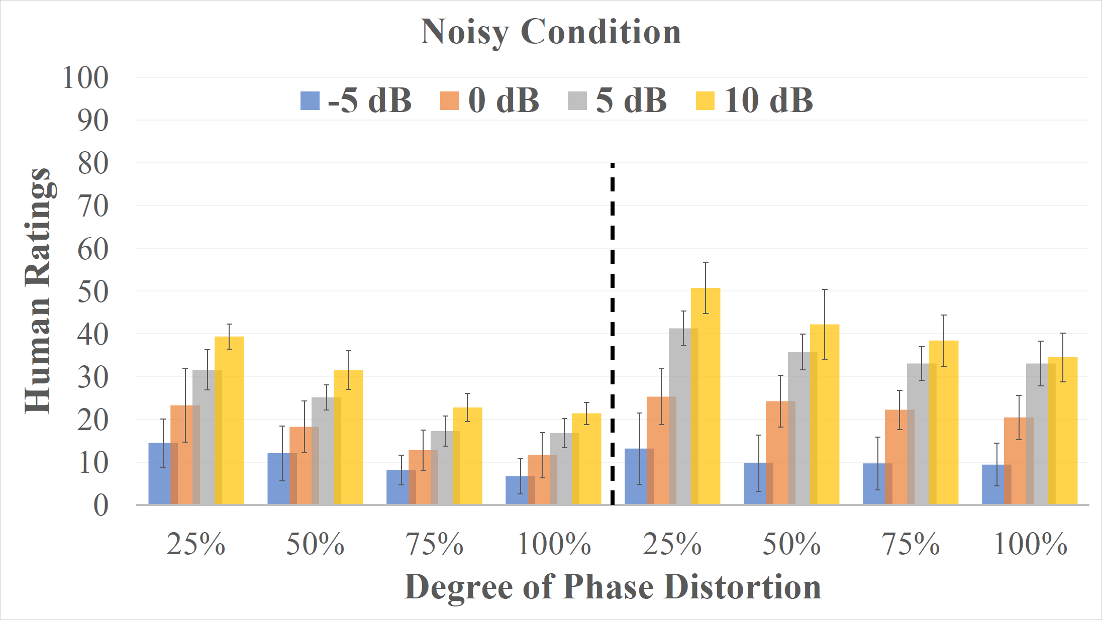
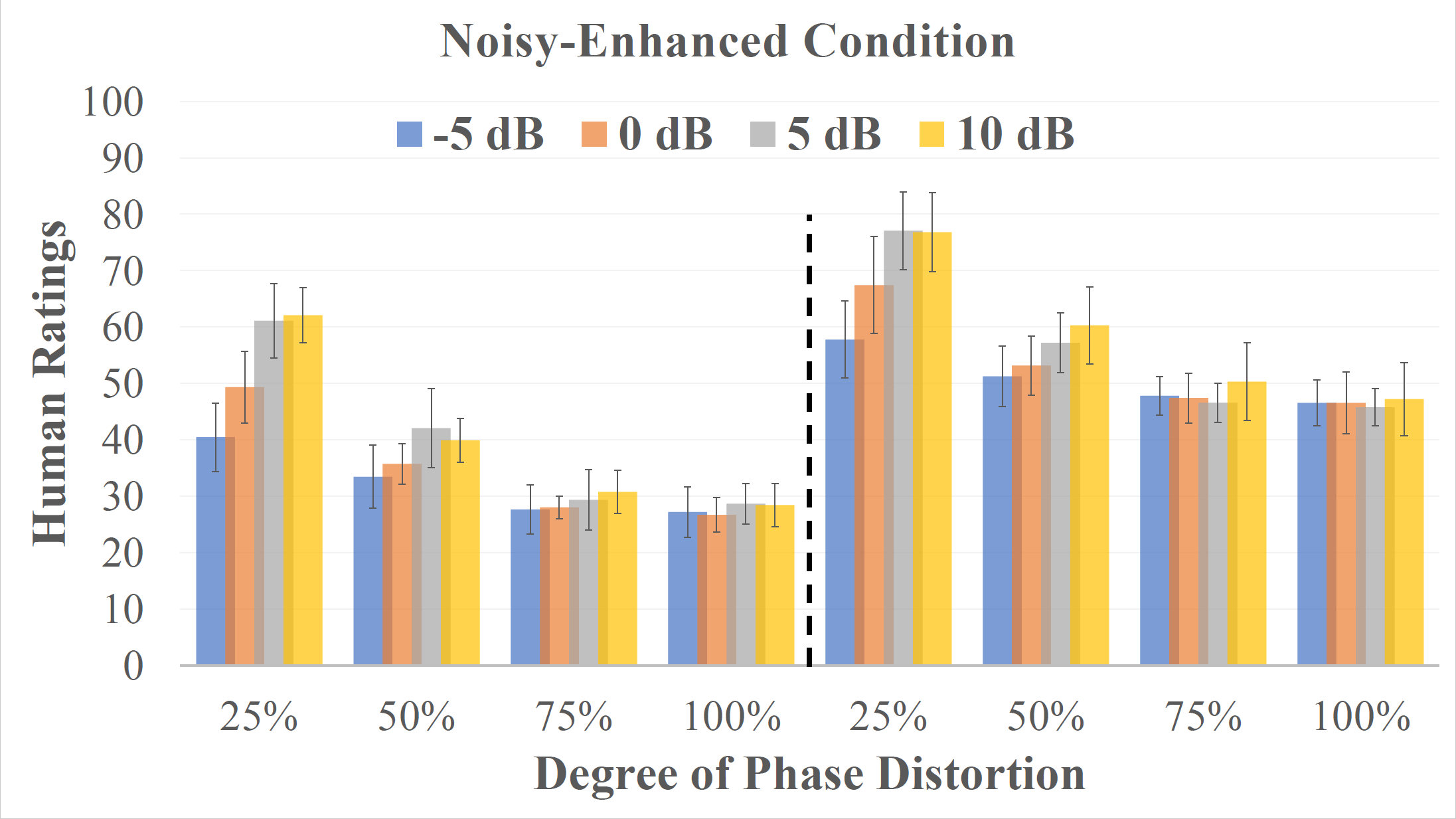
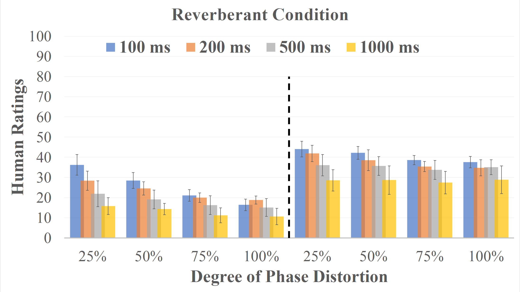
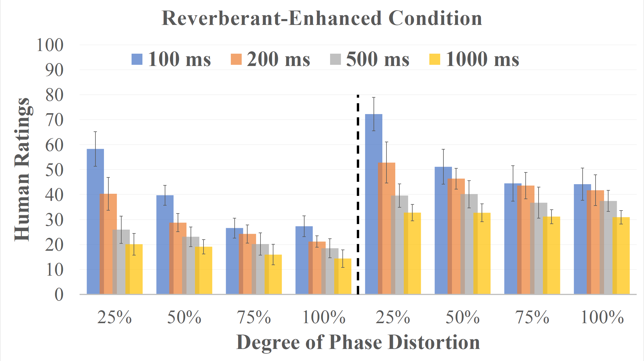
Quality ratings given by both normal and hearing-impaired listeners on speech signals in different conditions (i.e., from top-left to bot-right: (1). Noisy, (2). Noisy-enhanced, (3). Reverberant, (4). Reverberant-enhanced).

Hearing-impaired listeners tend to provide higher ratings for the same speech stimulus, corrupted by either background noise or reverberation, than NH listeners. Following phase-insensitive enhancement, HI and NH listeners can differentiate the degree of phase distortion that remained in the enhanced speech, indicating potential benefits from phase-sensitive enhancement techniques. Possible reasons for them to notice the phase distortions: (1) they have good TFS sensitivity, or (2) TFS and phase cues are weighed higher for quality tasks as compared to recognition tasks.

References:

• [1]. Y. Wang, A. Narayanan, and D. Wang, “On training targets for supervised speech separation,” IEEE/ACM transactions on audio, speech, and language processing, vol. 22, no. 12, pp. 1849–1858, 2014.
• [2]. F. Weninger, J. R. Hershey, J. Le Roux, and B. Schuller, “Discriminatively trained recurrent neural networks for single-channel speech separation,” in 2014 IEEE Global Conference on Signal and Information Processing (GlobalSIP). IEEE, 2014, pp. 577–581.
• [3]. R. S. ITU, “Recommendation bs. 1534-2: Method for the subjec-tive assessment of intermediate quality level of audio systems,” 2014.
• [4]. J. B. Allen and D. A. Berkley, “Image method for efficiently simulating small-room acoustics,” The Journal of the Acoustical Society of America, vol. 65, no. 4, pp. 943–950, 1979. [Online].Available: https://doi.org/10.1121/1.382599

×

Complex Ratio Masking

The below text provides information about a past project for speech enhancement. This page serves as a summary of the approach and results. For full details, please check out the papers that are referenced below. You can also view the above video by Prof. Donald Williamson for a general overview of the approach.

• D. Williamson and D. L. Wang, "Time-frequency masking in the complex domain for speech dereverberation and denoising," IEEE/ACM Trans. on Audio, Speech, and Lang. Process. (IEEE TASLP) , vol. 25, pp 1492-1501, 2017. [PDF]
• D. Williamson and D. L. Wang, "Speech Dereverberation and Denoising using Complex Ratio Masks," in Proc. IEEE International Conference on Acoustics, Speech, and Signal Processing (ICASSP) , pp. 5590-5594, 2017. [PDF]
• D. Williamson, Y. Wang, and D. L. Wang, "Complex ratio masking for monaural speech separation," IEEE/ACM Trans. on Audio, Speech, and Lang. Process. (IEEE TASLP), vol. 24, pp. 483-492, 2016. [PDF]
• D. Williamson, Y. Wang, and D. L. Wang, "Complex ratio masking for joint enhancement of magnitude and phase," in Proc. IEEE International Conference on Acoustics, Speech, and Signal Processing (ICASSP), pp. 5220-5224, 2016. [PDF]

To refer to these algorithms in a publication, please refer to the first reference below for speech enhancement involving additive noise, and the latter reference for the reverberant case.

• D. Williamson, Y. Wang, and D. L. Wang, "Complex ratio masking for monaural speech separation," IEEE/ACM Trans. on Audio, Speech, and Lang. Process. (IEEE TASLP), vol. 24, pp. 483-492, 2016. [PDF]
• D. Williamson and D. L. Wang, "Time-frequency masking in the complex domain for speech dereverberation and denoising," IEEE/ACM Trans. on Audio, Speech, and Lang. Process. (IEEE TASLP) , vol. 25, pp 1492-1501, 2017. [PDF]

Abstract

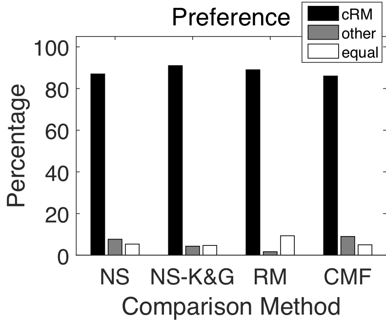
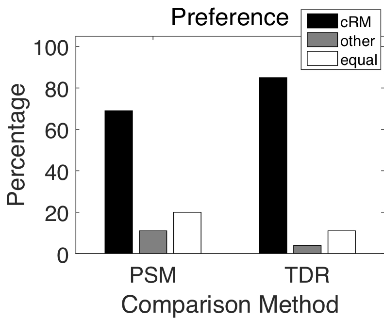
Speech separation systems usually operate on the short-time Fourier transform (STFT) of noisy speech, and enhance only the magnitude spectrum while leaving the phase spectrum unchanged. This is done because there was a belief that the phase spectrum is unimportant for speech enhancement. Recent studies, however, suggest that phase is important for perceptual quality, leading some researchers to consider magnitude and phase spectrum enhancements. We present a supervised monaural speech separation approach that simultaneously enhances the magnitude and phase spectra by operating in the complex domain. Our approach uses a deep neural network to estimate the real and imaginary components of the ideal ratio mask defined in the complex domain. We report separation results for the proposed method and compare them to related systems. The proposed approach improves over other methods when evaluated with several objective metrics, including the perceptual evaluation of speech quality (PESQ), and a listening test where subjects prefer the proposed approach with at least a 69% rate.

Background

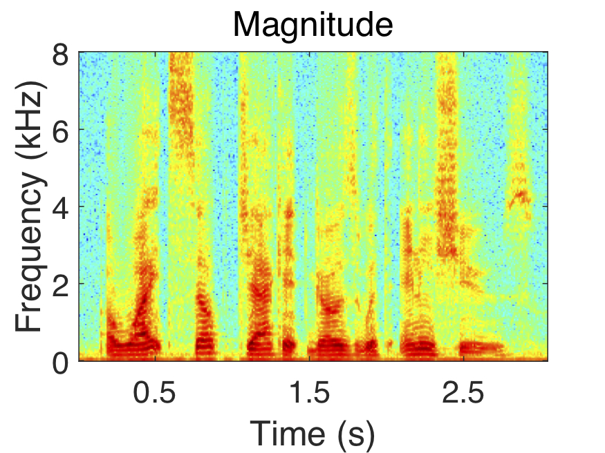
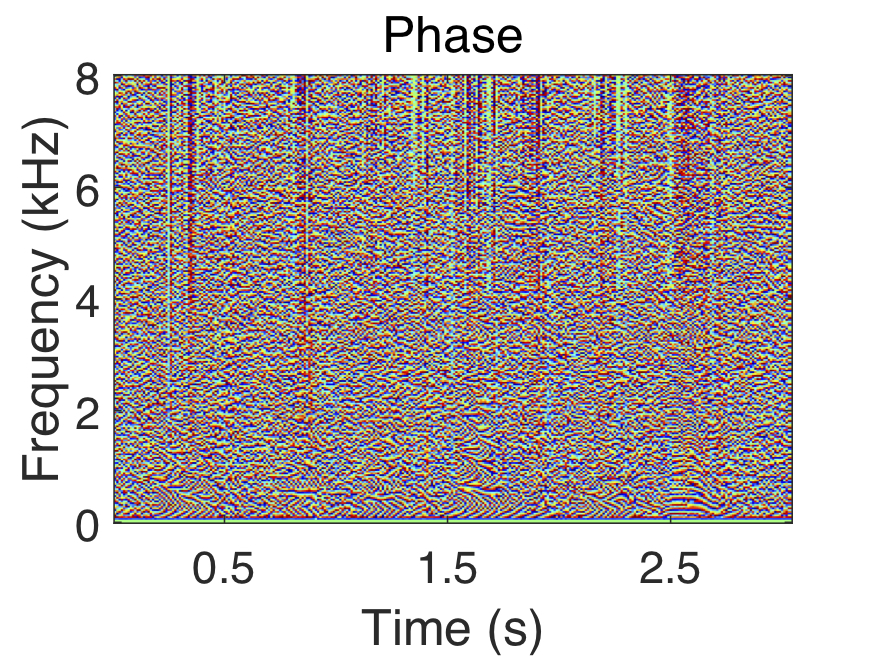
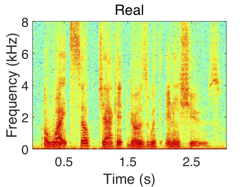
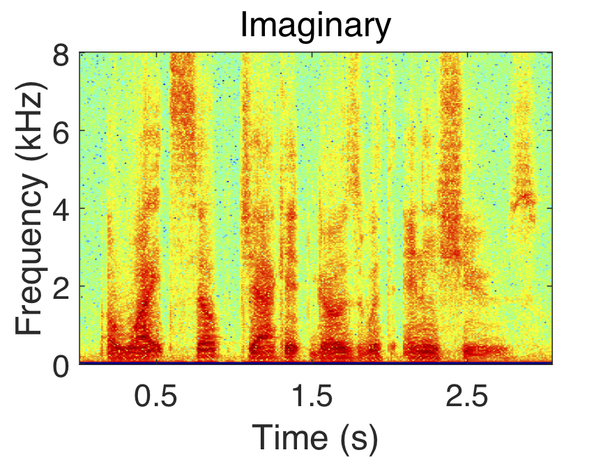
Polar coordinates (i.e. magnitude and phase) are commonly used when enhancing the short-time Fourier transform (STFT) of noisy speech. In this case, the STFT of noisy speech is represented as the product of its magnitude response and the complex exponential of its phase response. Mathematically, this is denoted as $S_{t,f} = |S_{t,f}|e^{i\Theta_{t,f}}$, where $S_{t,f}$ is the STFT, $|S_{t,f}|$ is the magnitude response, $\Theta_{t,f}$ is the phase response, $t$ is the time index, and $f$ is the frequency index.

As an alternative to using polar coordinates, the STFT can be expressed in Cartesian coordinates, using the expansion of the complex exponential. This results in the following expression: $S_{t,f} = |S_{t,f}|cos(\Theta_{t,f}) + i|S_{t,f}|sin(\Theta_{t,f})$. The first portion of the right-hand side of the equation is denoted as the real component (e.g. $S_r$), while the latter expression on the right-hand side of the equation (excluding the '$i$') is denoted as the imaginary component (e.g. $S_i$). We denote this cartesian representation as the complex domain.

The STFT components of a speech signal in polar and complex coordinates are shown above. Notice how the phase response appears random, while the magnitude, real, and imaginary components exhibit clear structure.

Complex Ratio Mask

Our goal is to derive a complex ratio mask that, when applied to the STFT of noisy speech, produces the STFT of clean speech. In other words, we want to find a complex mask that when multtplied with the noisy speech spectrum, results in the clean speech spectrum. Mathematically, this is represented as: $S_{t,f} = M_{t,f}\times Y_{t,f}$, where $M_{t,f}$ denotes the mask we want to compute.

Rearranging the terms in the above expression, we note that the mask can be computed from the spectra of the clean and noisy speech signals (e.g. $M_{t,f} = S_{t,f} / Y_{t,f}$). This mask is complex and will thus have a real and imaginary component. These components, denoted $M_r$ and $M_i$, can be computed directly from the real and imaginary components of the clean and noisy speech sigals.

$M_r = \frac{Y_rS_r + Y_iS_i}{Y_r^2 + Y_i^2}$

$M_i = \frac{Y_rS_i - Y_iS_r}{Y_r^2 + Y_i^2}$

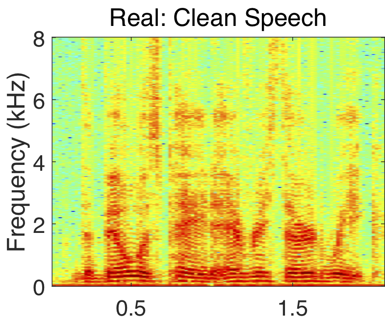
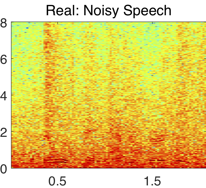
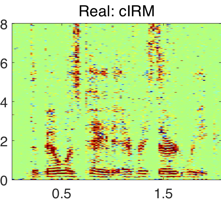
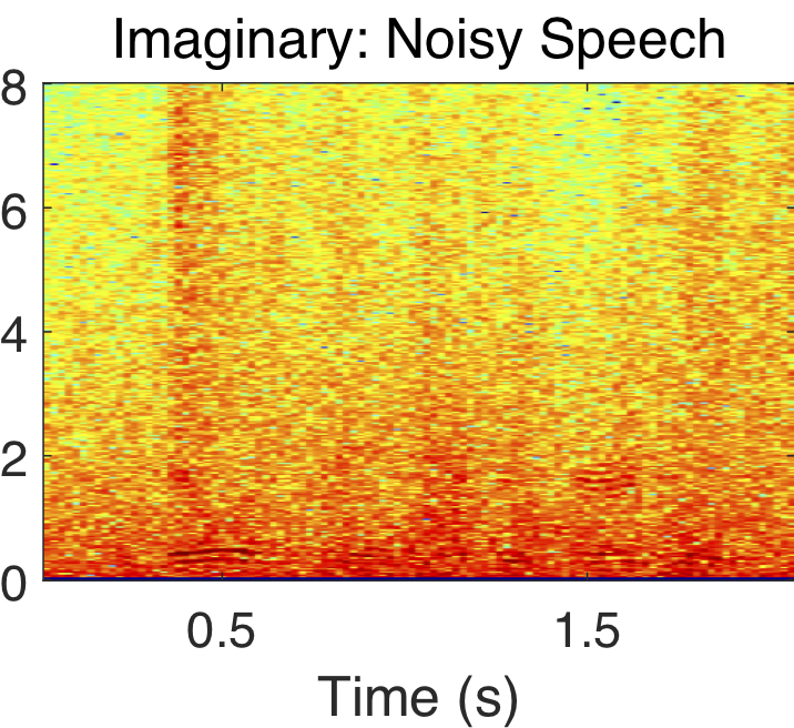
This mask is denoted as the complex ideal ratio mask (cIRM). Example real and imaginary components of a clean speech, noisy speech and its cIRM are shown above. Note that it is considered ideal, since it assumes that the clean speech spectra is available, which is not the case during testing. Thus, the cIRM must be estimated in order for enhancement to occur during testing. The deep neural network (DNN) shown below depicts how the cIRM is estimated from a noisy speech input signal. The DNN has three hidden layers and one output layer that is divided into to parts. One part of the output layer is used for estimating the real component of the cIRM, while the other portion estimates the imaginary component of the cIRM. The estimated complex mask is denoted as the complex ratio mask (cRM), hence it is no longer ideal.

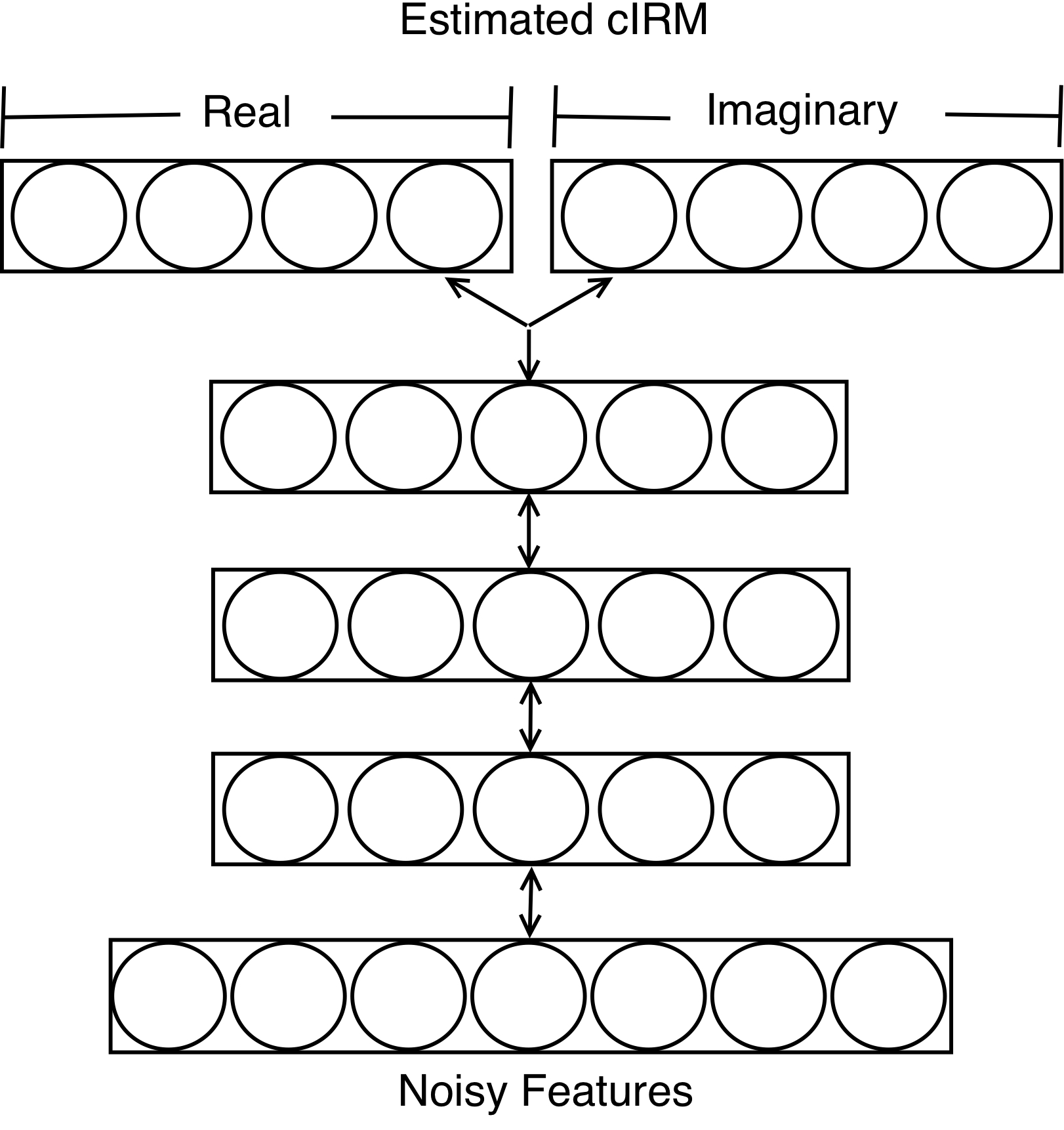
During testing, the estimated mask is applied to the STFT of noisy speech, resulting in an estimate of clean speech.

Results

The enhanced speech signals from different approaches are evaluated with the perceptual evaluation of speech quality (PESQ). The average PESQ scores for these approaches are shown in the table below, where higher scores indicate better performance. `cRM' denotes the proposed complex ratio masking approach. The 'Mixture' combines speech with four different types of noise (e.g. SSN, Cafe, Babble, or Factory).

	SSN	Cafe	Babble	Factory
Mixture	1.86	1.78	1.88	1.73
RM	2.31	2.16	2.34	2.23
cRM	2.52	2.32	2.35	2.41
PSM	2.44	2.23	2.41	2.33
TDR	2.38	2.27	2.32	2.33

Audio examples for the proposed cRM approach are below.

In addition to the objective results, we conducted a listening study to let human subjects compare pairs of signals. For each pair of signals, the participant is instructed to select one of three options: signal A is preferred, signal B is preferred, or the qualities of the signals are approximately identical. The listeners are instructed to play each signal at least once. The preferred method is given a score of +1 and the other is given a score of −1. A score of 0 is given to both signals if the participants deems that the qualities are approximately identical.

The listening study results are summarized in the figures below. The preference scores, shown in the two figures, show that the cRM approach is prefered at least 69% of the time as compared to comparison approaches.

×

Nulla viverra pharetra se, eget pulvinar neque pharetra ac int. placerat placerat dolor.

×

Nulla viverra pharetra se, eget pulvinar neque pharetra ac int. placerat placerat dolor.

×

Nulla viverra pharetra se, eget pulvinar neque pharetra ac int. placerat placerat dolor.

×

Nulla viverra pharetra se, eget pulvinar neque pharetra ac int. placerat placerat dolor.

×